How To Freeze the Top Row in Google Sheets

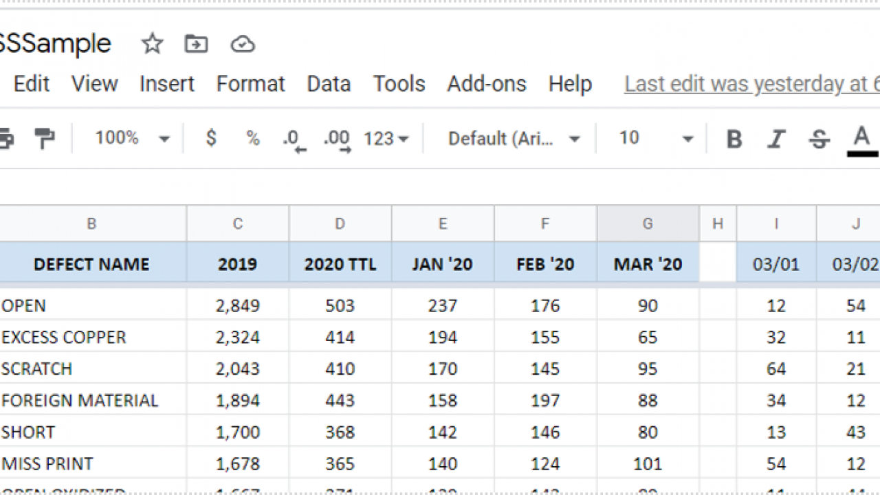
If you have to manage large spreadsheets or compare data within them, the ability to freeze a row or column can make life much easier. Depending on how the sheet is laid out, the top row can contain vital category headers or other information while the first column can contain the data necessary to identify cell data. Knowing how to freeze the top row in Google Sheets, or columns for that matter can help make short work of your analysis.

I tend to shift between Google Sheets and Excel depending on what my clients use. Some prefer the open source and cloud nature of Sheets while some prefer the security and enhanced features of Excel. I tend to prefer Excel because it feels better but they are both the same at their heart.

The methods you use to freeze rows and columns in Google Sheets differs slightly depending on what device you use to do it. Using a web browser is slightly different than using a mobile device. The examples here are from the browser version of Sheets. If you’re using mobile, most of these functions are accessed through the context menu.

Freeze the top row in Google Sheets

Freezing rows is useful for data comparison as this row usually contains column headers. Having them remain while you scroll down a large spreadsheet can help make sense of the data. Here’s how to do it.

Open your Sheet within your browser.
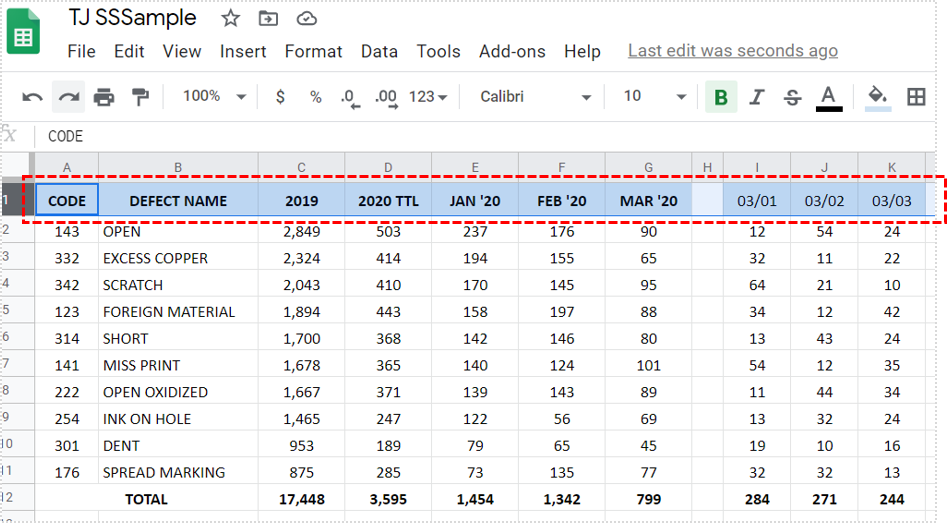
Select the row you want to freeze.
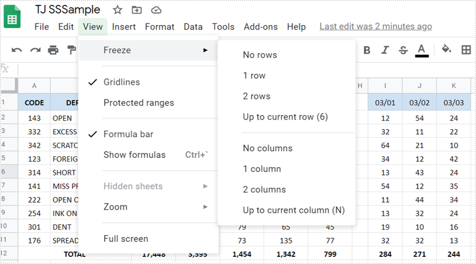
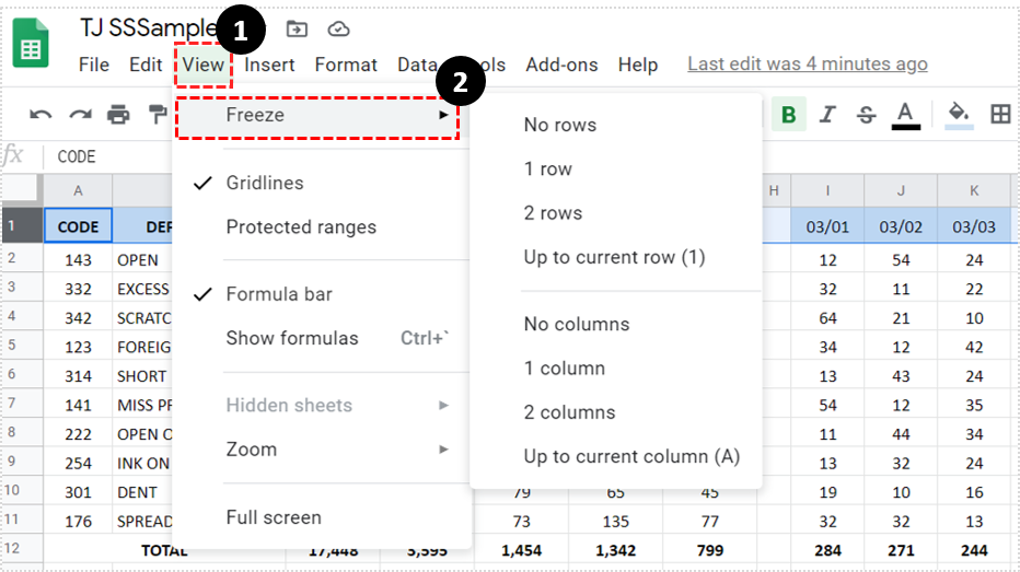
Select View and then Freeze.
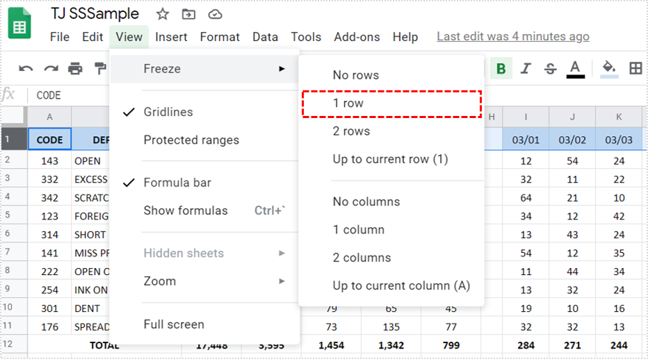
Select 1 row.

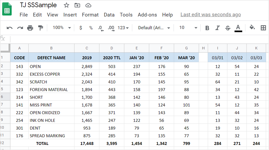
You should see a gray line appear underneath the row you froze. Scroll down the page and that row should remain in place while the rest scrolls as normal.
If you’re using a mobile device, you should tap the screen to select the row then tap again to bring up the context menu. You would then select the options from that menu. The same goes for freezing multiple rows, columns and for unfreezing rows or columns.

Freeze multiple rows in Google Sheets

If your data requires more than a single row, you can freeze multiple rows in Google Sheets. This is useful when comparing specific rows within a sheet.

Select the row below the one you want to freeze.
Select View and then Freeze.
Select Up to current row.

For example, if you wanted to freeze the top three rows, select row 3 and then View and Freeze. You should see ‘Up to current row (3)’. Select that and your rows will freeze. As far as I know, you can only freeze sequential rows. You cannot select different rows within a single sheet and freeze those.

Freeze a column in Google Sheets

Columns can also contain comparative data so it is useful to freeze those too. This is especially true for larger spreadsheets where category data is within column 1 and/or 2 and you have to scroll across so it disappears. Here’s how to freeze a column into place.

Select the column you want to freeze.
Select View and then Freeze.
Select 1 column.

If you select the column header, the entire column is highlighted. Then you select View and Freeze just like when you froze a row.

Freeze multiple columns in Google Sheets

You use the same commands to freeze multiple columns in Google Sheets. The only difference is that you select entire columns by their header letter or name instead of the row.

Select the columns you want to freeze.
Select View and then Freeze.
Select Up to current column.

For example, if you wanted to freeze the first two columns, select them and then View and Freeze. You should see ‘Up to current column (2)’.

Freeze columns and rows in Google Sheets

You can also freeze columns and rows in Google Sheets to make it easier to compare data across the entire spreadsheet. Essentially you repeat the instructions for freezing a row and then for freezing a column. The gray lines appear beside and underneath each and you’re done. I won’t repeat the instructions here, just freeze a row and then freeze a column as above.

To unfreeze rows or columns in Google Sheets

When you selected View and Freeze, you will also have noticed the option to freeze No rows or No columns. This is how you unfreeze a row or column. It may be an inelegant way to label it but the end result is the same.