How to Lock a Row in Google Sheets

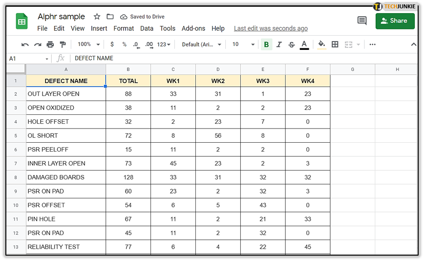
Google Sheets made sharing and organizing information less stressful, partially because it offers features like locking a row or a column. When your spreadsheet has too many rows and columns, navigation can become harder.

That’s why locking or freezing how it’s commonly called, a row or a column makes it easier to read the data in your spreadsheet. In this article, we’re going to show you how to do that.

Locking Rows and Columns in Google Sheets

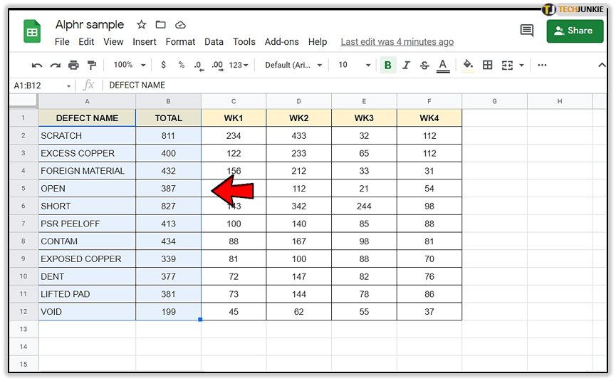
When you freeze or lock rows and columns in Google Sheets, it sets them in place, and they will not move. When dealing with a spreadsheet with too much data to keep track of, freezing rows and columns allows you to manage the document a little better.

In the majority of cases, you only need to lock the first column or row. But you can also freeze others that come after it. To lock a row or column, you only need three steps:

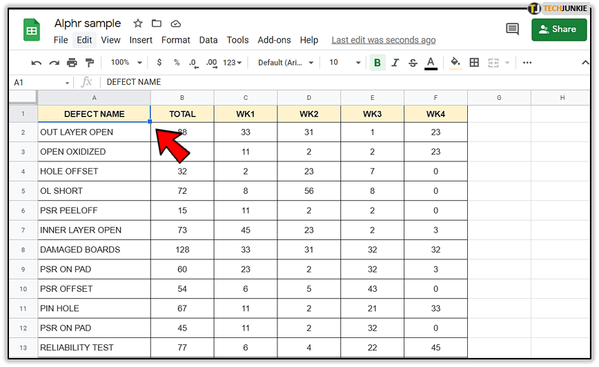
Select one cell in a row or column you want to lock.
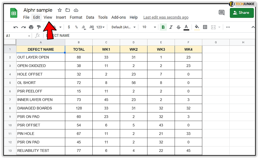
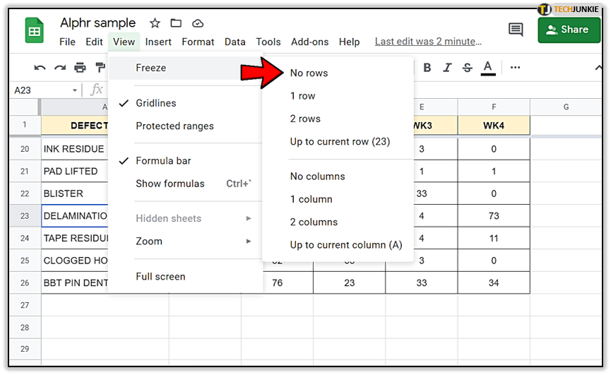
Go to the Google Sheets toolbar and click on “View.”
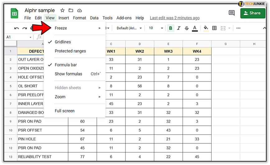
Select the “Freeze” option from the drop-down menu.
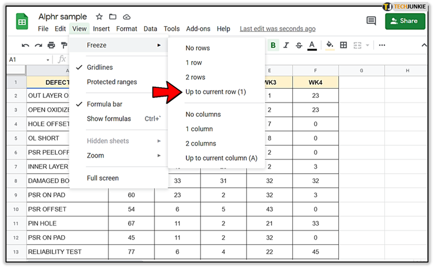
Choose “Up to Current Column” or “Up to Current Row,” which will lock every row or column up to the selected cell.

Once your rows and columns are locked, you can move around the spreadsheet, and they will stay in place. When you need to refer to them, you won’t have to navigate back to find them.

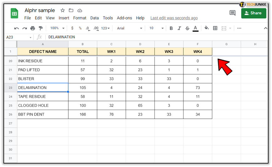
You’ll see a grey cell border that will better divide the locked and unlocked cells. In case you need to unlock rows and columns, go back to the “View>Freeze” option in the toolbar and select either “No Columns” or “Now Rows.”

Hiding Rows and Columns in Google Sheets

Sometimes you don’t need to lock the row or a column, and you also don’t need to refer to them while working on your spreadsheet. Instead of removing them, you can hide cells and rows temporarily. To do that, follow these steps:

Open Google Sheets in your browser.
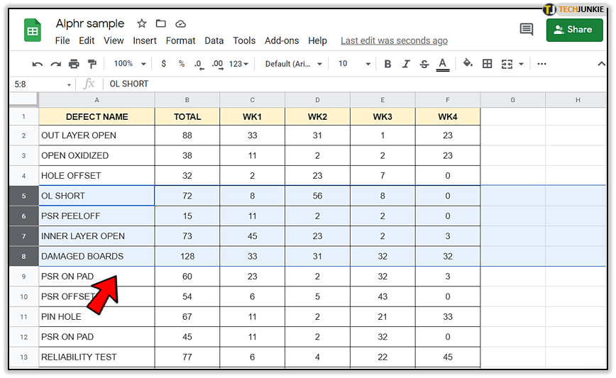
Select a row or a column you want to hide and highlight it.
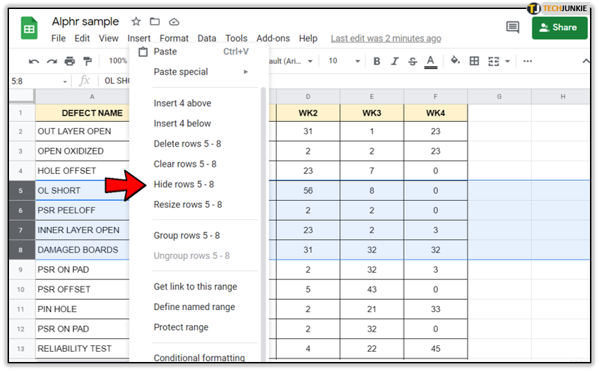
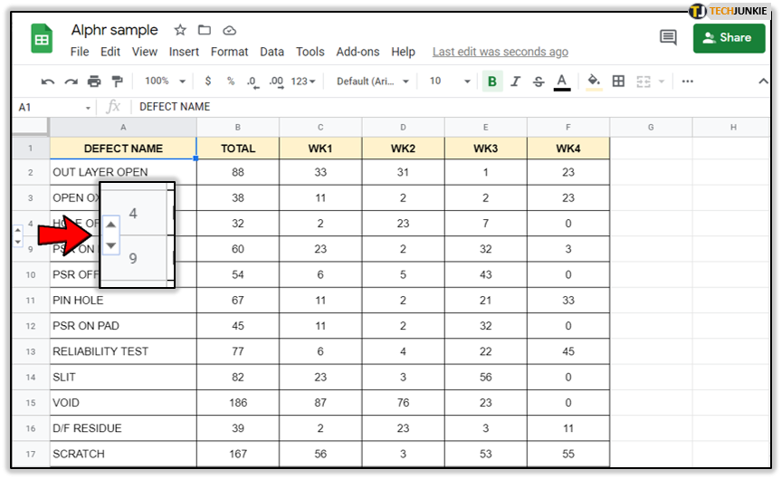
Right-click and then choose “Hide row” or “Hide column” from the menu. You’ll see an arrow over the now hidden column or row.

If you want to unhide the row or a column, all you need to do is click on that arrow.

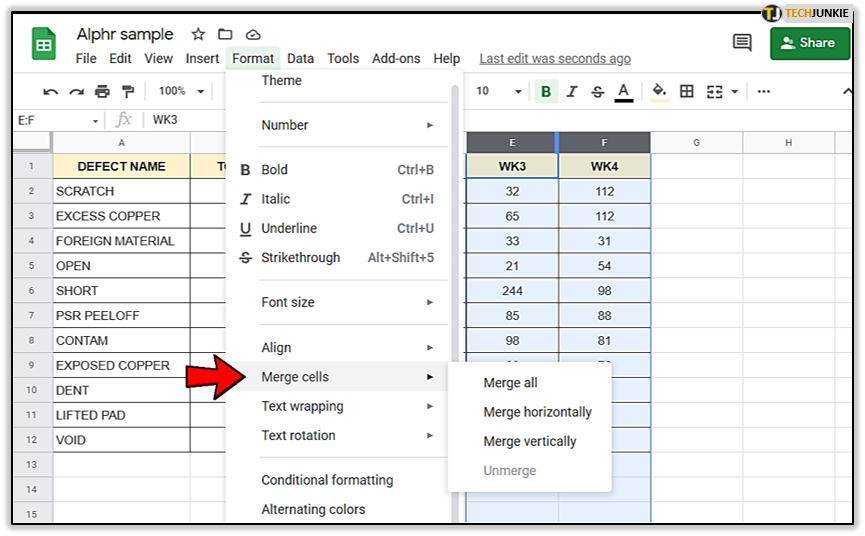
Also, if you want to merge rows or columns, that takes a few clicks, too. Select the rows and columns you want to join and go to the Google Sheets toolbar. Select “Format>Merge Cells,” and that’s all there is to it.

How to Lock Cells and Protect Google Sheets

In some cases, all you need is to lock a few cells in the entire spreadsheet. This feature in Google Sheets is aimed explicitly towards protecting certain parts of your document from modification. If you don’t want particular data edited or erased, locking a cell or cells is essential. Here’s how you do it:

Open Google Sheets and select a cell or range of cells you want to protect.
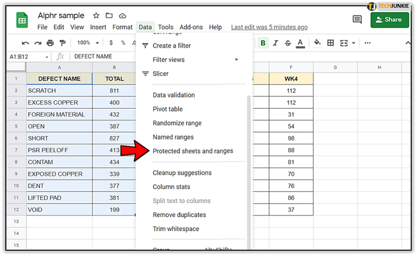
In the toolbar, go to “Data” and then select “Protected sheets and ranges.”
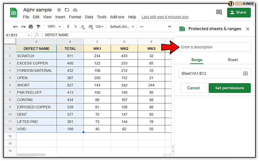
You’ll have the option to name the range, which we recommend for better navigation.
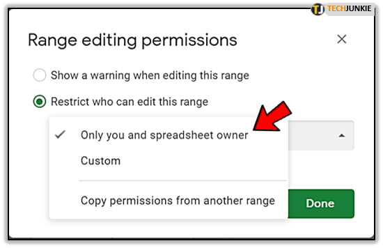
Select “Set permissions” then choose the option from the menu. You can either choose “Restrict who can edit this range” or “Only you.”

That way, you’ll make sure that only the collaborators you trust, or only you, can modify the cell or range in question.

Managing Your Google Sheets Efficiently

Nothing quite compares to the panic of realizing data is missing from your spreadsheet. Or that someone modified it incorrectly. That’s why Google Sheets protection matters. It ensures that every little bit of info is in its place always.

Locking or freezing rows and columns will save you a lot of time when working on a massive spreadsheet. Also, if you don’t need to use them at the moment, you can always hide any row or column you want.

Have you ever locked a cell, row, or a column in Google Sheets? Do you hide rows and columns sometimes? Let us know in the comments.