How to Freeze Multiple Rows or Columns in Google Sheets

Even if you organize your Google Sheet file with alternating colors, working with a large data set can be challenging. You constantly have to scroll through the spreadsheet to see all the data. Sometimes, you’d want to keep track of some of the data as you scroll further into the spreadsheet. This is possible by freezing the required rows. Wondering how to do this? Follow this guide to learn how.

What Happens When You Freeze in Google Sheets?

When you freeze cells or rows in sheets, the particular data will remain on-screen even if you scroll down in the sheet. This is very helpful when working with a lot of data, and you need to explore parts of the file. Frozen cells are also visible to others when they open the file.

Also, note that frozen rows remain in the same position even when you sort the data in the spreadsheet using a filter. 

How to Freeze Multiple Rows in Google Sheets on the Web

Luckily, you don’t need any third-party app or extension to freeze rows in Google Sheets. Also, the process of freezing single or multiple rows is the same. 

1. Open your spreadsheet in Google Sheets.
2. Select the row you want to freeze.
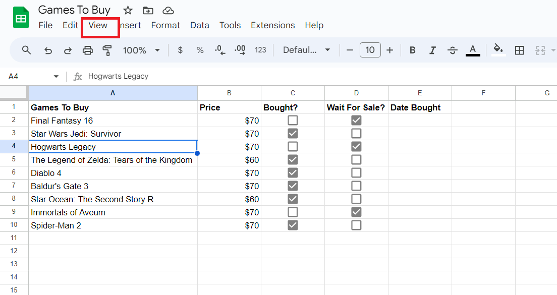
3. Click View from the toolbar at the top.
   
   
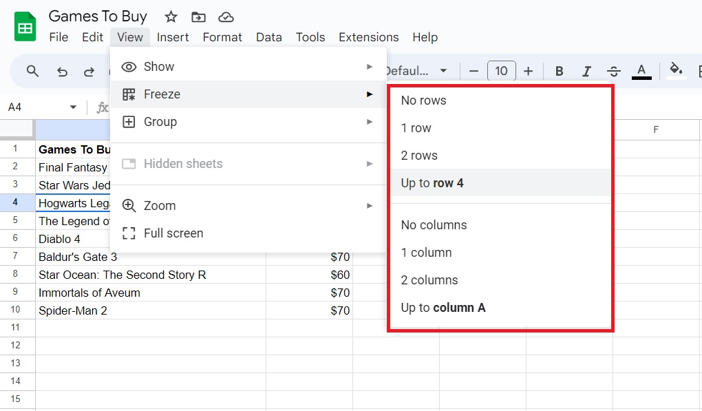
4. Select Freeze.
5. Choose what rows you want to freeze from the selection.
   

Once done, you should see a thick line that separates the frozen rows from the rest of the sheet. Regardless of where you go in the file, you’ll be able to see the fixed rows at the top.

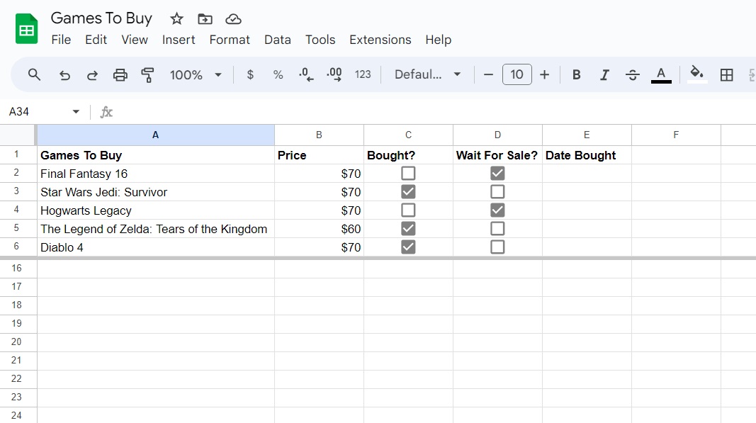
You can also freeze columns by selecting them from the Freeze menu. If you freeze by column, it should look like this:

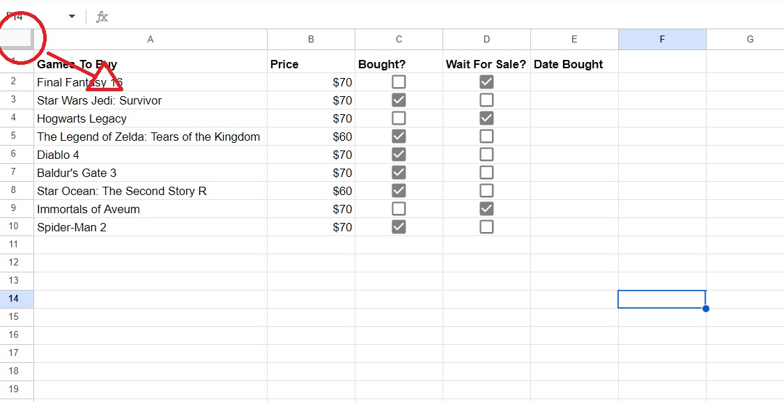
Alternatively, you can drag the freeze pane from the top right portion of the spreadsheet. Doing this will allow you to freeze the area where you dragged the pane to.

How to Unfreeze Rows in Google Sheets

Once you’re done freezing the data, you can unfreeze them anytime. Just make sure to follow these steps.

1. Open the spreadsheet in Google Sheets.
2. Select the row you want to freeze.
3. Click View.
   
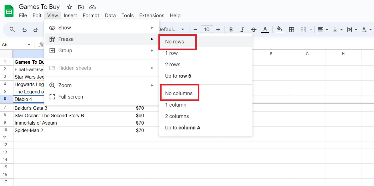
4. Select Freeze and then choose No Rows (or No Columns if you froze columns).
   

If you are inserting a calendar in Google Sheets, you should freeze the top row for easy navigation.

How to Freeze Multiple Rows or Columns in Google Sheets From Android or iPhone

If you’re working on a spreadsheet using the Google Sheets app on your phone, you can freeze rows or columns directly from the mobile app. You don’t have to switch to your PC for this simple task.

1. Open your spreadsheet in Google Sheets.
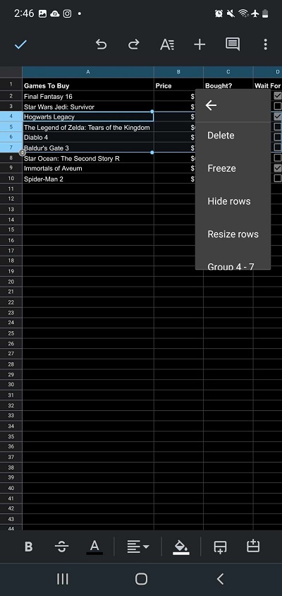
2. Tap the row number (or column letter) of the cells you want to freeze.
3. Touch and hold the highlighted rows or columns.
4. Select the three-dot icon.
   
   
5. Tap Freeze.
   
   

You can unfreeze the cells by going to the same menu and selecting Unfreeze.

Freezing Cells Make Managing Long Spreadsheets Easier

This little trick is beneficial, especially when it comes to spreadsheets that have loads of data. Do note that frozen cells are shared with everyone who has access to the Google Sheets file, making it easier for them to work on the spreadsheet, too. Next up, you might want to learn how to view who’s accessing your Google Docs or Sheets file.

FAQs