How To Link Data to Another Tab in Google Sheets

With its numerous add-ons, templates, and seamless integration with Microsoft Excel, Google Sheets has become an indispensable tool for students, professionals, and even just people looking to better organize their music collection. While it may not be quite as powerful as Excel, it is a great free alternative for those who prefer to stick with Google services.

Maybe you’ve been using it for a while now and are ready to up your game from Data Dabbler to Google Sheets Master. If so, there are two simple tricks the pros use that will take your spreadsheets to the next level. They both involve linking cells to other data and are fairly simple to implement.

The first is linking data to another tab, the second is pulling in data from another sheet or workbook — both of which can be very helpful in a wide variety of circumstances.

Let’s walk through the procedures so that you can take advantage of these features for yourself.

Link to Another Tab in Google Sheets

First, let’s take a look at how you can link to another tab in Google Sheets.

The steps to linking a cell to another tab are easy and straightforward:

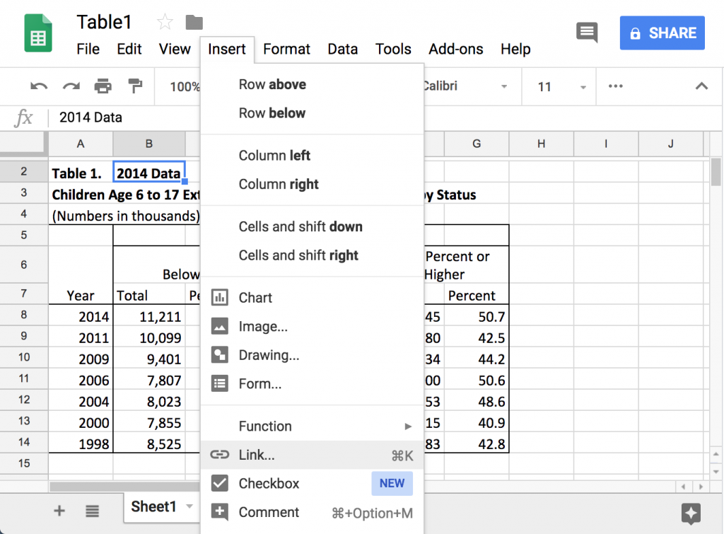
First, select a cell in your worksheet. It could be an empty cell or a cell that already has data. From the ‘Insert’ menu, select ‘Link.’ In the screenshot below, I’m selecting the cell at the top with the data “2014 Data.”

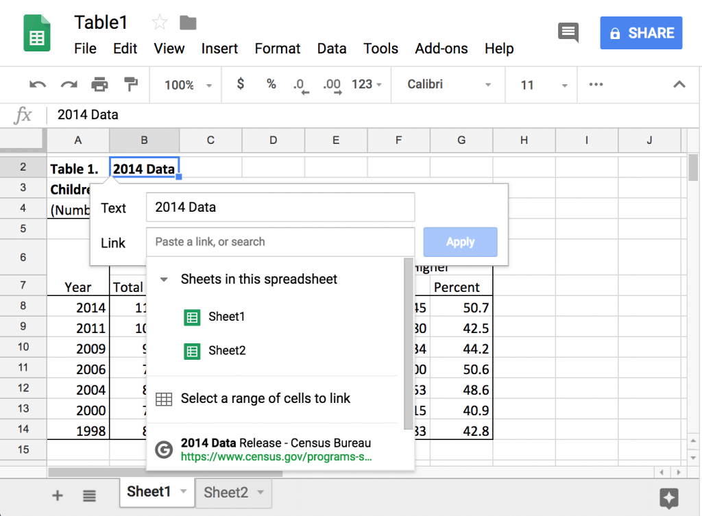
A dialog box will appear with a few options. It will ask if you want to link to “Sheets in this spreadsheet” (that’s another tab), or “Select a range of cells to link.” And Google being Google, it may also try to be clever and guess some other sources you might want to link to.

You’ll notice in the screenshot below, at the very bottom, Google is asking if I’d like to link to census.gov because it notices that’s where I grabbed this data from. This feature can be very helpful for keeping track of your sources when creating documents.

But for our purposes, let’s start by just linking to “Sheet2” because we’re already on “Sheet1.”

You’ll see the cell you selected will become a hyperlink. Now, whenever you click that cell, a pop-up will appear with a URL. Click on that URL and it will bring you to “Sheet2,” or whatever sheet you selected!

Now, let’s try the other option: selecting a range of cells. When we choose this option, another dialog will appear that says “What data?” (Pro tip: You can click and drag this dialog box to move it out of the way.)

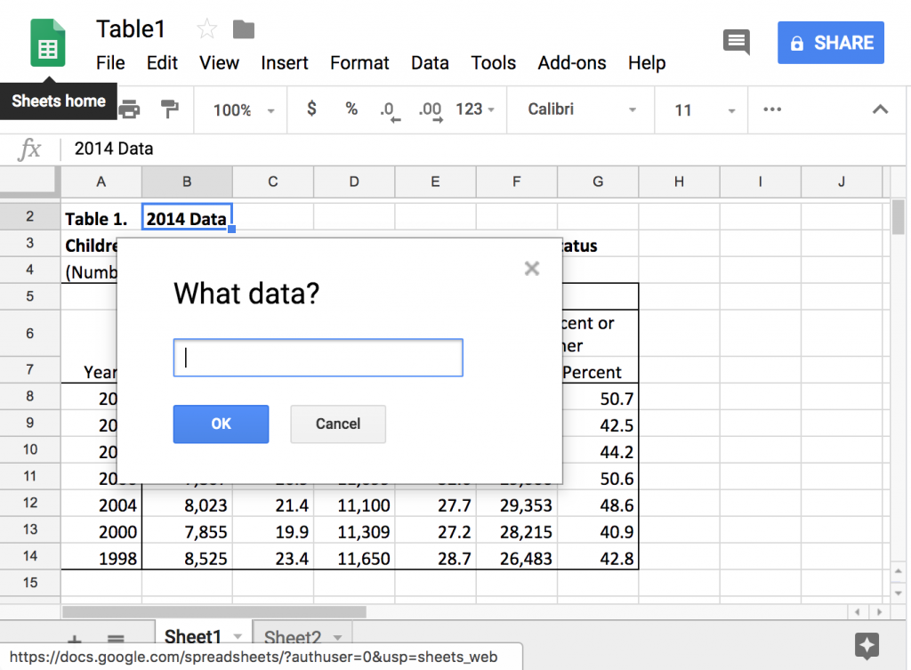
Now, you can either manually input the range of cells you want to link to, or you can click and drag a range of cells. In the below screenshot, I’ve selected all the data in row 8.

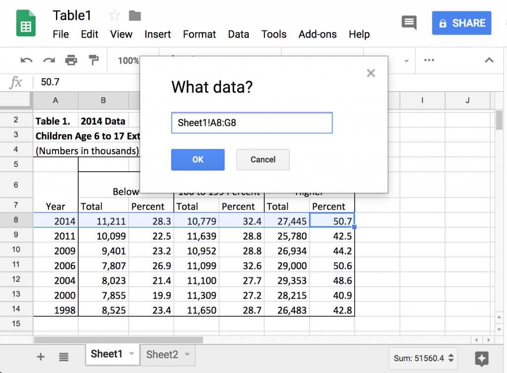
Now, whenever I click on the relevant cell, a pop-up link will appear, and when I click that link, all the data in row 8 will be selected. This can be very useful if your spreadsheet has a set of data that you’re constantly needing to select.

Link to Another Workbook in Google Sheets

What if you need to link to another workbook instead of another tab?

Linking to a workbook in Google Sheets is another advanced technique, and you can think of it as being almost like the opposite of inserting a link to another tab or range of cells. Instead of creating a link that will take us somewhere else, we’re creating a link that will pull in data from somewhere else. Unfortunately, this method requires a bit of manual coding, but don’t fret—it’s actually quite simple.

Linking to another workbook requires the use of the IMPORTRANGE function. When you use this function, you’re manually telling Google Sheets to go look for some data somewhere else and grab it.

If you want, you can activate this function by selecting the Insert menu, and then navigating to Function/Google/IMPORTRANGE. This will automatically insert the beginning of the code you need. But it’s probably even simpler to just do it manually. Start with the equals sign—that tells Google Sheets you’re about to input a function, rather than just data. Then type IMPORTRANGE.

The next thing Google Sheets will need to know is where you’re pulling the data from, and this happens in two parts. The first part is the worksheet, and the next is the actual cell or range of cells. These two pieces of information are each contained in quotation marks, and the whole thing is placed in parentheses. So in my case, I want to import data from a cell on Sheet2 into a cell on Sheet1.

Let’s just select the URL of our worksheet. If you wanted, you could select the URL of another worksheet. Then, we’ll paste that URL into our IMPORTRANGE function, and follow with the cell we want to grab, which in my case is cell G:21. The whole thing will look like this:

=IMPORTRANGE(“https://docs.google.com/spreadsheets/d/1PXYv00mWphBzvknmEY2JwcPqabdFgRA6nhZfaRjFA7w/edit#gid=261974994“, “sheet2!G21“)

You’ll notice we have an equals sign followed by IMPORTRANGE, and then the URL, the sheet and cell number both in quotation marks, and it’s all enclosed in parentheses. I’ve color-coded the three different parts to help you identify each element. This is what it will look like in your browser:

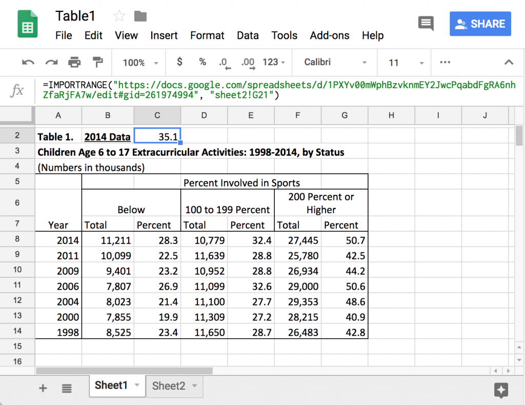
After you enter the function, you’ll probably see a red exclamation point in the cell. When you click on the cell, you’ll see an error message telling you the worksheets need to be linked, and a pop-up button will appear asking you if you want to link them. Once you allow the sheets to be linked, you’ll be good to go, and the cell will grab the data from the other sheet.

If you want to, you can also select a range of cells separated by a colon, like this: “sheet2!G10:G21”. This is telling Google Sheets to grab all the data from the G column that ranges between rows 10 and 21. But if you do this, just be sure the cell you’re importing this data into has enough space. In my example above, there is already data in the cells below my selected cell, C2, so Google Sheets wouldn’t allow me to import that range.

Learn More Ways to Use Google Sheets

Google Sheets is a very powerful, intuitive, and, best of all, free program for creating detailed spreadsheets. However, it can be difficult to figure out how to maximize its potential on your own.

Fortunately, here at TechJunkie, we have numerous articles to help you get the most out of Google Sheets, including How To Calculate Time in Google Sheets, How To Subtract in Google Sheets with a Formula, and How to Enable Dark Mode on Google Sheets.

Got any other ways to link Google Sheets or workbooks to each other? Tell us about them below if you do!