How to Rename Columns in the Google Sheets App

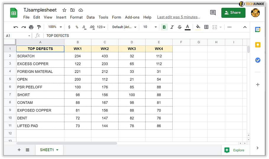
Google Sheets has a specific way to label the first column and row headers. It uses numbers to specify the rows, and the letters A-Z to sort the columns.

These headers are particularly convenient if you have tens, hundreds, or even thousands of rows. As they’re always visible at the top, you don’t have to scroll all the way up (which becomes too time-consuming). However, if you try to change the names of these headers, you’ll encounter a stumbling block.

Fortunately, there’s a way around this issue – thanks to the ‘freeze’ feature. Let’s find out more about it.

Why Is Freezing Rows and Columns Important?

The first column and row of your Google spreadsheet will always be visible when you scroll. So even if you reach row 800, you’ll still be able to see which column it belongs to.

By default, the columns that you see are labeled A, B, C, etc. Because of this, you’ll need to remember what header ‘A’ represents, as well as add the value to the row. It would be much easier, therefore, to rename that ‘A’ column into the item it represents. But, as aforementioned, you can’t modify the first header of columns and rows.

That’s where the ‘freeze’ column feature comes in handy. Instead of changing the name of column ‘A’, you can freeze the column below it, and have it act as the header. This way, even when you scroll down, the column name will still be visible.

This will make it significantly easier to keep track of your data and help avoid accidental mistakes while you’re entering it into particular columns. You’ll find out how to freeze rows and columns on your Sheets app in the following section.

How to Freeze a Row

Freezing a row in Sheets is relatively easy on both the PC version and mobile app.

Freeze a Row in Sheets on PC

If you’re using a PC web browser version of Google sheets, do this to freeze the rows and columns:

1. Open the Google Sheets document.
   
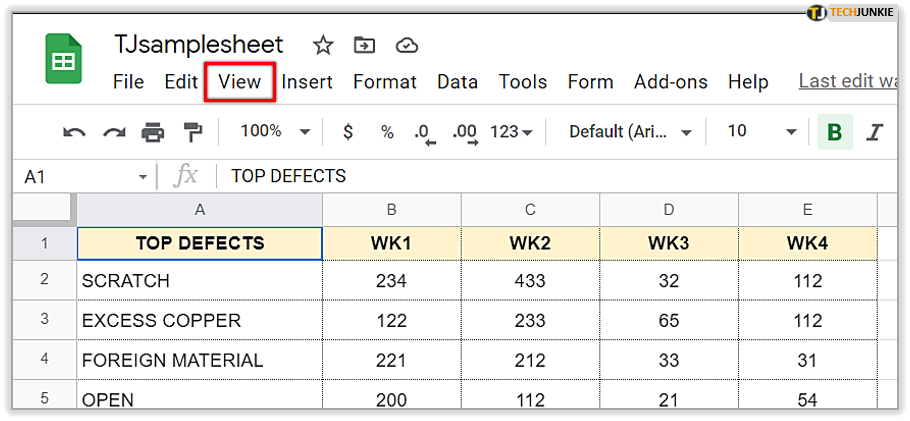
2. Click the ‘View’ menu on the bar at the top of the screen.
   
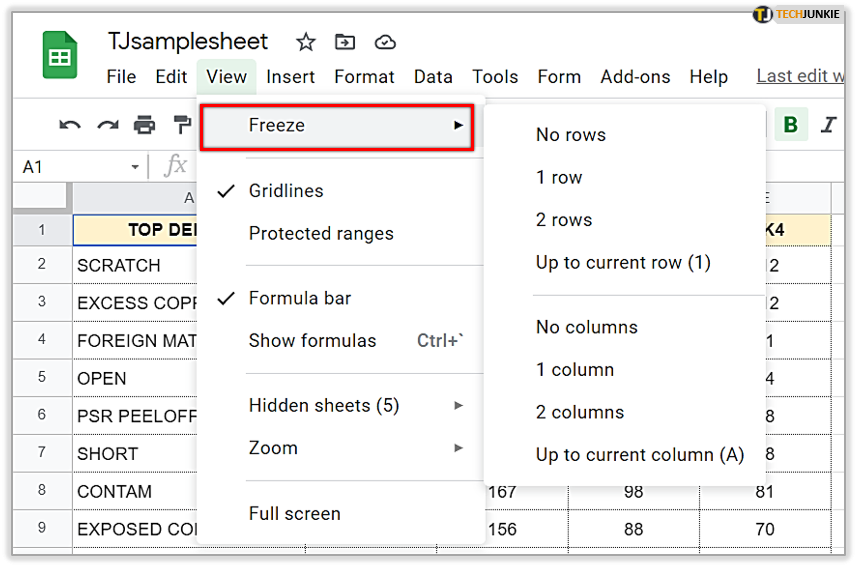
3. Hover over the ‘Freeze’ menu with your mouse. A new menu will appear.
   
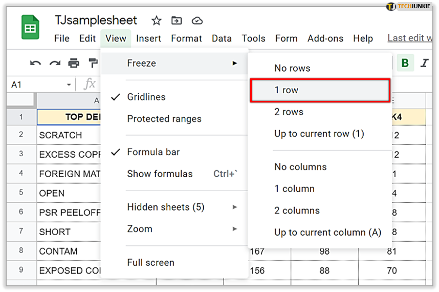
4. Choose either ‘1 row,’ ‘2 rows,’ or ‘Up to current row’. The ‘Up to current row’ option will freeze all the rows above and including the row that is currently highlighted. For example, if you click the row ‘13’, you’ll freeze all the rows including the thirteenth.
   

Freeze a Column in Sheets on Mobile App

Freezing a row on a mobile app is a bit different. Here’s what you need to do:

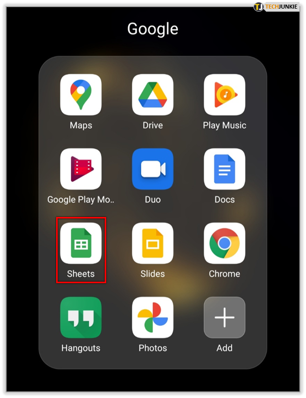
1. Open the Sheets app on your Android/iPhone device.
   
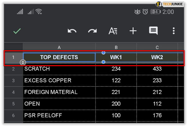
2. Tap and hold the row that you want to freeze.
   
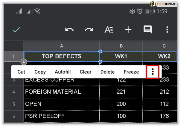
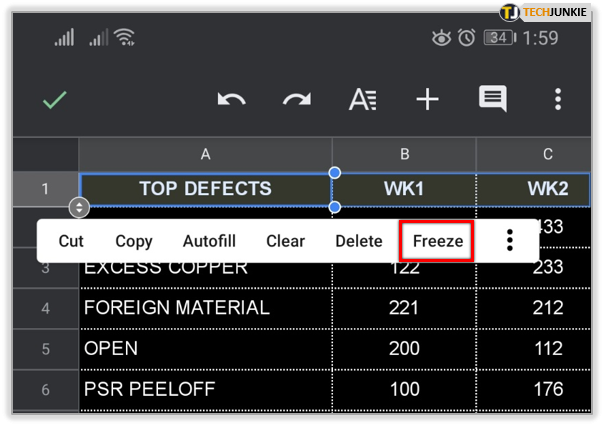
3. If the Freeze option doesn’t show, Select the ‘more icon’ (three horizontal dots) when the new box appears.
   
4. Press ‘Freeze.’
   

Once you select the number of rows you want to freeze, you’ll see the grey line dividing that row from the rest of the document.

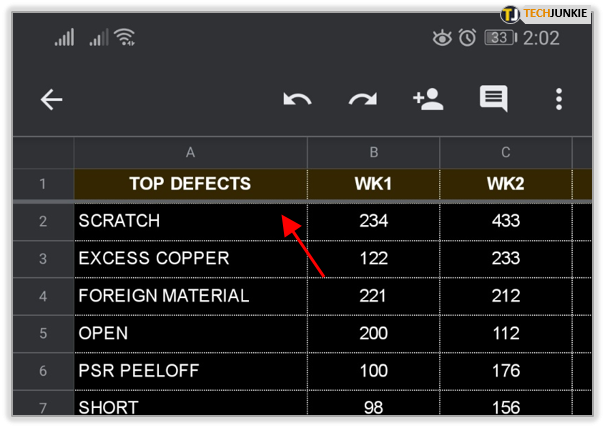
Users rarely freeze more than one row, particularly to solve the issue stated in this article. Therefore, if you want the columns from your first row to represent the headers of the rows, there’s no need to freeze two or more.

Rename the Columns in Google Sheets App

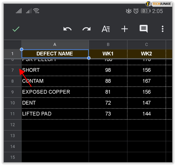
Now that you’ve frozen the row that will represent the column headers, you can rename them and always be aware of which value they represent.

You can easily rename the column in Sheet app:

1. Open the Sheets app.
   
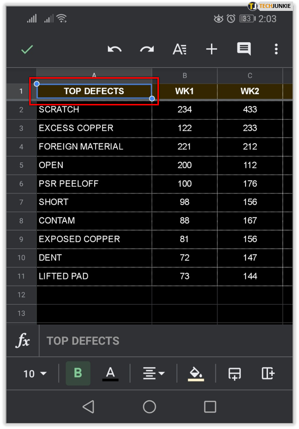
2. Tap the column that you want to rename.
   
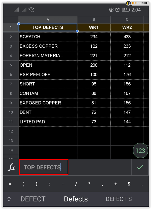
3. Type in the name at the field next to the ‘fx’ symbol. (Alternatively, you can just double-tap the column instead of steps 2 and 3).
   
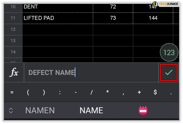
4. Tap the checkmark once you enter the name.
   

After you freeze the row and rename your columns, you can scroll down as much as you want, but the columns of the first row will always be visible. Thanks to this, you’ll hardly ever mix up the values of those columns.

What About Freezing Columns?

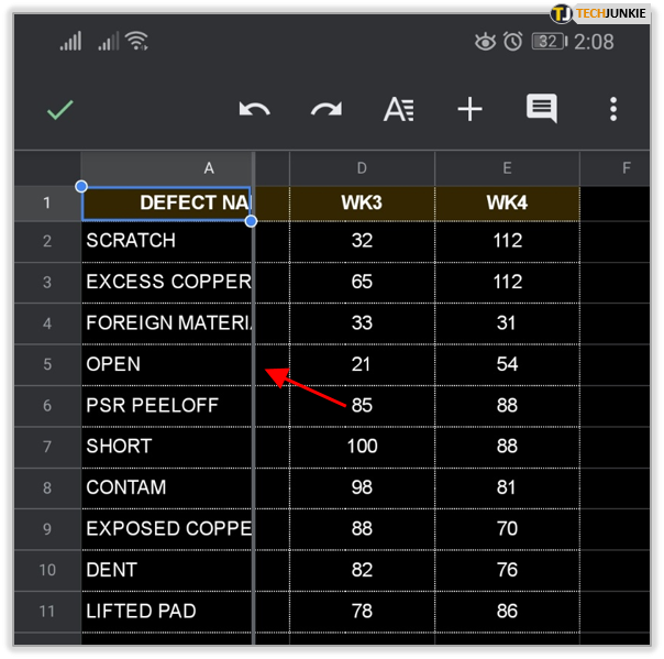
You can follow the same steps from the previous sections to freeze the columns along with (or instead of) rows. This will essentially do the opposite thing, as it will freeze one column and the first value of each row.

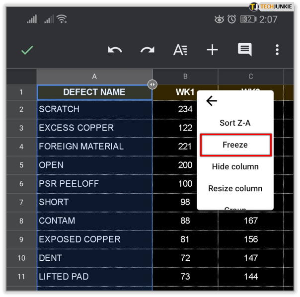
This way, each row of the first column will remain visible. This is useful if you’re inputting multiple values in separate columns, instead of separate rows. Therefore, when you move your spreadsheet document to the right, you’ll still know the value of the first cell in a row.

Freezing Rows– A Great Way to Avoid Mistakes

Renaming columns in your mobile app isn’t a big issue. Only when you want to rename the A-Z headers is it impossible. However, freezing rows essentially turns the columns below into the same thing.

Thanks to the freezing and renaming method described in this article, you can always keep track of the headers. This will save a lot of time that you’d otherwise spend on correcting the errors, which frequently happens when you can’t always see a proper column name.

Did you find this solution useful? Share your experiences in the comments section below.