How to VLOOKUP from Another Spreadsheet in Google Sheets Using IMPORTRANGE

VLOOKUP is a powerful tool to check the data in your spreadsheets. However, when you want to pull an item from a worksheet in another Workbook, you might run into problems. Luckily, you can use the IMPORTRANGE function in Google Sheets to solve this issue.

In this article, we’ll show you how to combine IMPORTRANGE with VLOOKUP. Plus, we’ll also provide additional tips that might help enhance your experience.

Using IMPORTRANGE – Step by Step Guide

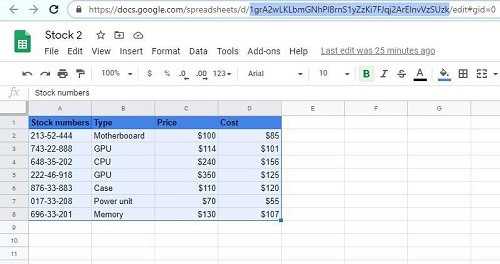
For the purposes of this article, we’ll use two workbooks from the computer hardware shop. Our goal is to pull the price data from the workbook “Stock 2” into “Stock 1”.

Start by copying the key from the “Stock 2” workbook URL. You only need the part that is between “/d/” and “/edit.” You can see it highlighted in the picture above.
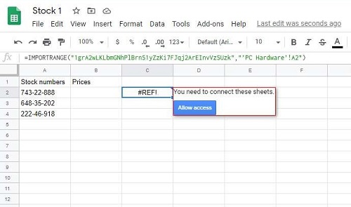
Now you can use the IMPORTRANGE function to connect “Stock 1” and “Stock 2” workbooks. As you want to import data from “Stock 2”, go into “Stock 1”, click on any field and implement the formula:

IMPORTRANGE (spreadsheet_key, range_string)

In our example, the formula is:

IMPORTRANGE(“1grA2wLKLbmGNhPlBrnS1yZzKi7FJqj2ArEInvVzSUzk”,”’PC Hardware’!A2″)

Note that when the name of the name sheet contains more than a single word, you’ll need to use single quotes.

After using the formula, you may need to wait before the data from “Stock 2 “loads. Once it’s done, you’ll receive the message, “You need to connect these sheets“. Now, click on “Allow access” to finish the process.

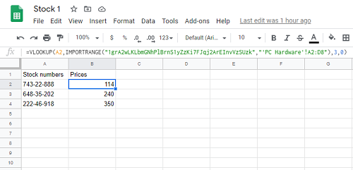
As workbooks are now connected, we can finally use VLOOKUP, by combining it with IMPORTRANGE. Delete the data in B2, and use this formula:

VLOOKUP(A2,IMPORTRANGE(“1grA2wLKLbmGNhPlBrnS1yZzKi7FJqj2ArEInvVzSUzk”,”‘PC Hardware’!A2:D8″),3,0)

What we implemented in our formula are range and index, while we used “0” for “is_sorted” syntax. Also, we didn’t have to define our range strictly. Instead of “A2:D8”, we could’ve used “A2:D”. That way, VLOOKUP checks every field in the “D” column. This solution is useful if you plan to add more data, as you won’t have to change the formula in “Stock 1”.

Enhance VLOOKUP and IMPORTRANGE Experience

When to Use “Issorted” Syntax?

The Is_Sorted syntax is FALSE by default, and we’re leaving it that way in our example. When using FALSE, Vlookup will search for exact matches. If there’s more than one correct value, it will use the first one. FALSE should be used if you don’t need sorting.

If the columns need to be sorted, for example, from smallest to the largest value, then you should use TRUE in your formula. In this case, Vlookup will try to find the closest value if there’s no exact match. If the closest value is bigger than search_key, the result won’t appear.

Use Wildcards with Vlookup in Google Sheets

We didn’t have that problem in our example, but sometimes you might not know the entire search key. Luckily, wildcards will assist you. It would help if you used Asterisk (*) when matching sequences of characters while the question mark (?) matches a single character.

Override VLOOKUP Limitation with Index Match Formula

Both in Excel and Google Sheets, VLOOKUP can’t look at its left and will return an error if the first column isn’t the search column. Use the following formula when needed

INDEX (return_range, MATCH(search_key, lookup_range, 0))

Index Match references the return column directly so that structural changes won’t affect it, unlike VLOOKUP. When you remove or insert a column inside, the Vlookup formula will become invalid, while Index Match won’t be affected. This function also works in Excel, but the arguments have different names.

VLOOKUP and IMPORTRANGE in Google Sheets and Excel: The Differences

Using VLOOKUP and IMPORTRANGE is almost the same in Google Sheets and Excel. However, there are four key differences:

While they work in the same way, formulas are defined differently in both apps. Google Sheets are considered more intuitive.

In Google Sheets, you’ll see the return value as you type formula. It will appear in the white box above the formula.

You can use wild characters with VLOOKUP only in Google Sheets.

In Google Sheets the overhead bar matches the color of the formula, making it easier to identify.

IMPORTRANGE to the Rescue

Using IMPORTRANGE with VLOOKUP gives you endless possibilities to combine the data in Google Sheets’ workbooks. As you’ve hopefully seen, formulas are intuitive, while the implementation of wildcard characters is better than in Excel. The only thing you might miss when working with a few workbooks is the side-by-side view that’s only in Microsoft Excel.

Do you often need to pull the data from a few workbooks at the same time? Have you used IMPORTRANGE in other spreadsheets? Let us know in the comments section below.